Week 3: Independence, Random Variables, and Distributions

Reading: Casella & Berger (C&B) §1.3 (independence, pp. 24–27) and §§1.4–1.6

Lecture	Date	Topics	C&B
3.1	Tue. Oct. 13	Independence of two and of several events; random variables; induced probability functions	§1.3 (end), §1.4
3.2	Thu. Oct. 15	Cumulative distribution functions; continuous and discrete random variables; identically distributed random variables; probability mass and density functions	§§1.5–1.6

Notation. Random variables are uppercase ($X$, $Y$); their realized values are lowercase ($x$, $y$). $\mathcal{X}$ is the range of $X$. $F_X$ is the cdf of $X$ and $f_X$ its pmf or pdf. $\mathcal{B}^1$ is the Borel sigma algebra on the real line: the smallest sigma algebra containing all intervals. $X \sim F_X(x)$ reads “$X$ is distributed as $F_X(x)$.”

Independence

Way of thinking. Translate intuition into equations.

1. Independence of two events

Sometimes learning $B$ tells us nothing about $A$: $P(A \mid B) = P(A)$. By Bayes’ rule (1.3.5) this implies $P(B \mid A) = P(B)$, and by the multiplication rule $P(A \cap B) = P(A) P(B)$. We take the symmetric version as the definition.

Definition 1.3.7. Two events, $A$ and $B$, are statistically independent if

\[P(A \cap B) = P(A)\, P(B). \tag{1.3.8}\]

This definition is symmetric in $A$ and $B$, does not require $P(B) > 0$, and extends to more than two events.

Example 1.3.8 (Chevalier de Méré). Is it a good bet that at least one six appears in 4 rolls of a die? By independence of the rolls,

\[P(\text{at least one 6 in 4 rolls}) = 1 - P(\text{no 6 in 4 rolls}) = 1 - \left( \frac{5}{6} \right)^4 \approx 0.518.\]

De Méré also bet on at least one double six in 24 rolls of two dice, reasoning that it should be equally likely. In fact $1 - (35/36)^{24} \approx 0.491$, a losing bet. His losses prompted the Pascal–Fermat correspondence of 1654, often taken as the birth of probability theory.

Theorem 1.3.9. If $A$ and $B$ are independent events, then the following pairs are also independent:

(a) $A$ and $B^c$,
(b) $A^c$ and $B$,
(c) $A^c$ and $B^c$.

Proof of (a). By Theorem 1.2.9(a) and independence,

\[P(A \cap B^c) = P(A) - P(A \cap B) = P(A) - P(A) P(B) = P(A) \big( 1 - P(B) \big) = P(A) P(B^c). \qquad \square\]

Parts (b) and (c) are Exercise 1.40.

Independent vs. disjoint. These are very different. If $P(A) > 0$ and $P(B) > 0$ and $A, B$ are disjoint, then $P(A \cap B) = 0 \ne P(A) P(B)$, so they are dependent: learning that $A$ occurred tells you $B$ did not (Exercise 1.39).

2. Independence of several events

What should it mean for $A$, $B$, and $C$ to be independent? Two natural guesses both fail.

Guess 1: $P(A \cap B \cap C) = P(A) P(B) P(C)$ is enough. False.

Example 1.3.10 (Tossing two dice). Roll two dice, with $S$ the 36 equally likely ordered pairs. Let $A$ = “doubles,” $B$ = “the sum is between 7 and 10,” and $C$ = “the sum is 2, 7, or 8.” Then $P(A) = 1/6$, $P(B) = 1/2$, $P(C) = 1/3$, and

\[P(A \cap B \cap C) = P(\lbrace (4,4) \rbrace) = \frac{1}{36} = \frac{1}{6} \cdot \frac{1}{2} \cdot \frac{1}{3}.\]

But $P(B \cap C) = P(\text{sum equals 7 or 8}) = 11/36 \ne P(B) P(C) = 1/6$. Similarly, $P(A \cap B) \ne P(A) P(B)$, so the triple product condition does not even guarantee pairwise independence.

Guess 2: pairwise independence is enough. False.

Example 1.3.11 (Letters). Let $S$ consist of the $3!$ permutations of the letters a, b, and c along with the three triples of each letter, each with probability $1/9$:

\[S = \lbrace aaa, \; bbb, \; ccc, \; abc, \; bca, \; cba, \; acb, \; bac, \; cab \rbrace.\]

Let $A_i$ = “the $i$th place in the triple is occupied by a.” Then $P(A_i) = 1/3$ and $P(A_i \cap A_j) = 1/9$ for all $i \ne j$, so the $A_i$ are pairwise independent. But $P(A_1 \cap A_2 \cap A_3) = P(\lbrace aaa \rbrace) = 1/9 \ne 1/27$.

Definition 1.3.12. A collection of events $A_1, \dots, A_n$ are mutually independent if for any subcollection $A_{i_1}, \dots, A_{i_k}$, we have

\[P\left( \bigcap_{j=1}^{k} A_{i_j} \right) = \prod_{j=1}^{k} P(A_{i_j}).\]

For three events that is four equations: three pairwise conditions plus the triple one. For $n$ events it is $2^n - n - 1$ equations.

Example 1.3.13 (Three coin tosses–I). Toss a coin three times, with sample space

\[S = \lbrace HHH, HHT, HTH, THH, TTH, THT, HTT, TTT \rbrace,\]

and assign probability $1/8$ to each point. Let $H_i$ = “toss $i$ is a head,” for example $H_1 = \lbrace HHH, HHT, HTH, HTT \rbrace$. Then $P(H_i) = 1/2$,

$P(H_1 \cap H_2 \cap H_3) = P(\lbrace HHH \rbrace) = \frac{1}{8} = \frac{1}{2} \cdot \frac{1}{2} \cdot \frac{1}{2},$ $P(H_1 \cap H_2) = P(\lbrace HHH, HHT \rbrace) = \frac{2}{8} = \frac{1}{2} \cdot \frac{1}{2},$

and similarly for the other pairs. So $H_1, H_2, H_3$ are mutually independent: a head on any toss has no effect on any other toss. Conversely, assigning $1/8$ to each point is the only probability model with $P(H_i) = 1/2$ and $H_1, H_2, H_3$ mutually independent. This is what “three independent tosses of a fair coin” means.

Check your understanding.

If $P(A) = 0.4$, $P(B) = 0.5$, and $A$, $B$ are independent, find $P(A \cup B)$.

Show answer

$P(A \cup B) = P(A) + P(B) - P(A) P(B) = 0.4 + 0.5 - 0.2 = 0.7$. Alternatively, by Theorem 1.3.9(c), $P(A \cup B) = 1 - P(A^c) P(B^c) = 1 - 0.6 \times 0.5 = 0.7$.
Show that if $P(B) = 1$, then $B$ is independent of every event $A$.

Show answer

$P(A \cap B^c) \le P(B^c) = 0$, so $P(A \cap B) = P(A) - P(A \cap B^c) = P(A) = P(A) P(B)$.
A system has three components that work independently, each with probability $0.9$. It works if at least one component works. What is the probability the system works?

Show answer

By Theorem 1.3.9 the complements are also mutually independent, so $P(\text{all fail}) = 0.1^3 = 0.001$ and $P(\text{system works}) = 0.999$.

Random Variables

Way of thinking. A random variable is neither random nor a variable: it is a function on the sample space.

3. Definition and examples

In many experiments it is easier to work with a summary than with the original sample space. Ask 50 people whether they agree (1) or disagree (0) with a statement. The sample space has $2^{50}$ elements, ordered strings of 0s and 1s. If all we care about is $X$ = the number of people who agree, the new sample space is just $\lbrace 0, 1, \dots, 50 \rbrace$.

Definition 1.4.1. A random variable is a function from a sample space $S$ into the real numbers.

Example 1.4.2 (Random variables). In some experiments random variables are implicitly used:

Experiment	Random variable
Toss two dice	$X$ = sum of the numbers
Toss a coin 25 times	$X$ = number of heads in 25 tosses
Apply different amounts of fertilizer to corn plants	$X$ = yield/acre

4. The induced probability function

Defining a random variable also defines a new sample space, its range $\mathcal{X}$. We must check that the probability function $P$ on $S$ can be used for $X$.

Suppose $S = \lbrace s_1, \dots, s_n \rbrace$ with probability function $P$, and $X$ has range $\mathcal{X} = \lbrace x_1, \dots, x_m \rbrace$. We observe $X = x_i$ if and only if the outcome is an $s_j \in S$ with $X(s_j) = x_i$. So we define

\[P_X(X = x_i) = P\big( \lbrace s_j \in S : X(s_j) = x_i \rbrace \big). \tag{1.4.1}\]

$P_X$ is an induced probability function on $\mathcal{X}$, defined in terms of $P$. It satisfies the Kolmogorov Axioms (Exercise 1.45). Because of (1.4.1) we simply write $P(X = x_i)$ rather than $P_X(X = x_i)$.

A note on notation. Random variables are always denoted with uppercase letters and their realized values (or range) with the corresponding lowercase letters. The random variable $X$ can take the value $x$.

Example 1.4.3 (Three coin tosses–II). Toss a fair coin three times (Example 1.3.13) and let $X$ = number of heads.

$s$	HHH	HHT	HTH	THH	TTH	THT	HTT	TTT
$X(s)$	3	2	2	2	1	1	1	0

The range is $\mathcal{X} = \lbrace 0, 1, 2, 3 \rbrace$. With probability $1/8$ on each point, counting gives

$x$	0	1	2	3
$P_X(X = x)$	$1/8$	$3/8$	$3/8$	$1/8$

For example, $P_X(X = 1) = P(\lbrace HTT, THT, TTH \rbrace) = 3/8$.

Example 1.4.4 (Distribution of a random variable). We can find $P_X$ even without a complete listing. Let $S$ be the $2^{50}$ equally likely strings of 50 0s and 1s, $X$ = number of 1s, and $\mathcal{X} = \lbrace 0, 1, \dots, 50 \rbrace$. Then

$P_X(X = 27) = \frac{\text{number of strings with 27 1s}}{\text{number of strings}} = \frac{\binom{50}{27}}{2^{50}},$ and in general, $P_X(X = i) = \frac{\binom{50}{i}}{2^{50}}, \quad i \in \mathcal{X}.$

This is Week 2’s counting at work.

Uncountable range. If $\mathcal{X}$ is uncountable, we define $P_X$ in the same way as (1.4.1): for any set $A \subset \mathcal{X}$,

\[P_X(X \in A) = P\big( \lbrace s \in S : X(s) \in A \rbrace \big). \tag{1.4.2}\]

This is a legitimate probability function. (To be precise, (1.4.2) defines probabilities only for a certain sigma algebra of subsets of $\mathcal{X}$, the Borel sets. C&B do not dwell on this, and neither will we.)

The key picture. $\lbrace X \in A \rbrace$ is shorthand for the event $\lbrace s \in S : X(s) \in A \rbrace$, the inverse image of $A$ under $X$. Every probability statement about $X$ is a statement about an event in $S$.

Check your understanding.

Roll two fair dice and let $X$ = the sum. Write the event $\lbrace X = 4 \rbrace$ as a subset of $S$ and find $P(X = 4)$.

Show answer

$\lbrace X = 4 \rbrace = \lbrace (1,3), (2,2), (3,1) \rbrace$, so $P(X = 4) = 3/36 = 1/12$.
In Example 1.4.3, let $Y = X^2$. Is $Y$ a random variable? Find the range of $Y$ and $P(Y = 4)$.

Show answer

Yes: $Y(s) = X(s)^2$ is again a function from $S$ into the real numbers. Its range is $\lbrace 0, 1, 4, 9 \rbrace$ and $P(Y = 4) = P(X = 2) = 3/8$. Functions of random variables are the topic of Chapter 2.

Distribution Functions, Mass Functions, and Density Functions

Way of thinking. cdf vs. pdf

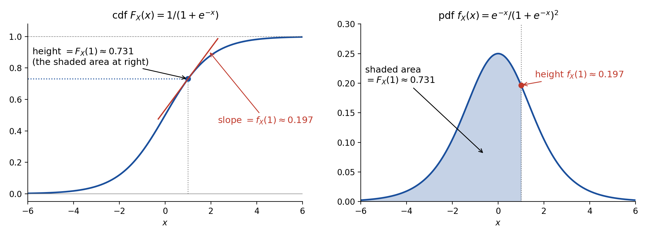
cdf vs. pdf of the logistic distribution

Figure. The cdf (left) and pdf (right) of the logistic distribution (Examples 1.5.5 and 1.6.4). The height of the cdf at $x$ equals the area under the pdf to the left of $x$: $F_X(x) = \int_{-\infty}^{x} f_X(t)\, dt$. Going back, the slope of the cdf at $x$ equals the height of the pdf: $f_X(x) = \frac{d}{dx} F_X(x)$. At $x = 1$: $F_X(1) \approx 0.731$ and $f_X(1) \approx 0.197$.

5. The cumulative distribution function

Definition 1.5.1. The cumulative distribution function or cdf of a random variable $X$, denoted by $F_X(x)$, is defined by

\[F_X(x) = P_X(X \le x), \quad \text{for all } x.\]

Example 1.5.2 (Tossing three coins). Toss three fair coins and let $X$ = number of heads. The cdf of $X$ is

\[F_X(x) = \begin{cases} 0 & \text{if } -\infty < x < 0 \\ \frac{1}{8} & \text{if } 0 \le x < 1 \\ \frac{1}{2} & \text{if } 1 \le x < 2 \\ \frac{7}{8} & \text{if } 2 \le x < 3 \\ 1 & \text{if } 3 \le x < \infty. \end{cases} \tag{1.5.1}\]

$F_X$ is defined for all real $x$, not just $x \in \mathcal{X} = \lbrace 0, 1, 2, 3 \rbrace$. For example, $F_X(2.5) = P(X \le 2.5) = P(X = 0, 1, \text{ or } 2) = 7/8$.
$F_X$ is a step function. It jumps at each $x_i \in \mathcal{X}$, and the size of the jump at $x_i$ is $P(X = x_i)$.
$F_X(x) = 0$ for $x < 0$ since $X$ cannot be negative, and $F_X(x) = 1$ for $x \ge 3$.

Right-continuity. At a jump point, $F_X$ takes the value at the top of the jump (note the inequalities $\le$ and $<$ in (1.5.1)). So $F_X$ is continuous when a point is approached from the right. This follows from the “$\le$” in the definition. Had we defined $F_X(x) = P_X(X < x)$, $F_X$ would be left-continuous. In general, the size of the jump at any point $x$ is

\[P(X = x) = F_X(x) - \lim_{t \uparrow x} F_X(t).\]

Theorem 1.5.3. The function $F(x)$ is a cdf if and only if the following three conditions hold:

a. $\lim_{x \to -\infty} F(x) = 0$ and $\lim_{x \to \infty} F(x) = 1$.
b. $F(x)$ is a nondecreasing function of $x$.
c. $F(x)$ is right-continuous; that is, for every number $x_0$, $\lim_{x \downarrow x_0} F(x) = F(x_0)$.

Outline of proof. Necessity (every cdf has these properties) follows by writing $F$ in terms of the probability function (Exercise 1.48). For example, (b) holds because $x_1 < x_2$ implies $\lbrace X \le x_1 \rbrace \subset \lbrace X \le x_2 \rbrace$, so $F(x_1) \le F(x_2)$ by Theorem 1.2.9(c). Parts (a) and (c) need the continuity of probability along monotone sequences of events. Sufficiency (any $F$ with these properties is the cdf of some random variable) is much harder: we must construct a sample space $S$, a probability function $P$ on $S$, and a random variable $X$ on $S$ whose cdf is $F$. $\square$

Why this theorem matters. To specify a distribution, we do not need to build $S$ and $P$ explicitly. Any function with properties (a)–(c) will do.

Example 1.5.4 (Tossing for a head). Toss a coin until a head appears, where $p$ = probability of a head on any given toss, and let $X$ = number of tosses required to get a head. For $x = 1, 2, \dots$,

\[P(X = x) = (1 - p)^{x-1} p, \tag{1.5.2}\]

since we need $x - 1$ tails followed by a head, and the tosses are independent. For any positive integer $x$,

\[P(X \le x) = \sum_{i=1}^{x} P(X = i) = \sum_{i=1}^{x} (1 - p)^{i-1} p. \tag{1.5.3}\]

Using the partial sum of the geometric series (Exercise 1.50),

\[\sum_{k=1}^{n} t^{k-1} = \frac{1 - t^n}{1 - t}, \quad t \ne 1, \tag{1.5.4}\]

we get

\[F_X(x) = P(X \le x) = \frac{1 - (1-p)^x}{1 - (1-p)}\, p = 1 - (1 - p)^x, \quad x = 1, 2, \dots.\]

Between the integers $F_X$ is flat, so for all real $x \ge 1$, $F_X(x) = 1 - (1 - p)^{\lfloor x \rfloor}$, and $F_X(x) = 0$ for $x < 1$.

If $0 < p < 1$, $F_X$ satisfies Theorem 1.5.3:

(a) $F_X(x) = 0$ for all $x < 0$, and $\lim_{x \to \infty} 1 - (1-p)^x = 1$.
(b) The sum in (1.5.3) contains more positive terms as $x$ increases.
(c) For any $x$, $F_X(x + \epsilon) = F_X(x)$ if $\epsilon > 0$ is small enough, so $\lim_{\epsilon \downarrow 0} F_X(x + \epsilon) = F_X(x)$.

This is the cdf of the geometric distribution (named after the series).

Example 1.5.5 (Continuous cdf). The function

\[F_X(x) = \frac{1}{1 + e^{-x}} \tag{1.5.5}\]

satisfies Theorem 1.5.3: $\lim_{x \to -\infty} F_X(x) = 0$ since $\lim_{x \to -\infty} e^{-x} = \infty$; $\lim_{x \to \infty} F_X(x) = 1$ since $\lim_{x \to \infty} e^{-x} = 0$; and

\[\frac{d}{dx} F_X(x) = \frac{e^{-x}}{(1 + e^{-x})^2} > 0,\]

so $F_X$ is increasing. It is not only right-continuous but continuous. This is a special case of the logistic distribution, the same function as the logistic (sigmoid) link in logistic regression.

Example 1.5.6 (Cdf with jumps). A cdf can mix continuous pieces and jumps. For some $\epsilon$ with $1 > \epsilon > 0$, let

\[F_Y(y) = \begin{cases} \dfrac{1 - \epsilon}{1 + e^{-y}} & \text{if } y < 0 \\[2ex] \epsilon + \dfrac{1 - \epsilon}{1 + e^{-y}} & \text{if } y \ge 0. \end{cases} \tag{1.5.6}\]

$F_Y$ has a jump of height $\epsilon$ at $y = 0$ and is otherwise continuous (Exercise 1.47). Think of a gauge whose reading could be any real number but that sometimes sticks at 0, with $\epsilon$ the probability that it sticks.

6. Continuous and discrete random variables

Definition 1.5.7. A random variable $X$ is continuous if $F_X(x)$ is a continuous function of $x$. A random variable $X$ is discrete if $F_X(x)$ is a step function of $x$.

So Examples 1.5.2 and 1.5.4 are discrete, Example 1.5.5 is continuous, and Example 1.5.6 is neither.

Definition 1.5.8. The random variables $X$ and $Y$ are identically distributed if, for every set $A \in \mathcal{B}^1$, $P(X \in A) = P(Y \in A)$.

Identically distributed does not mean equal: Definition 1.5.8 does not say $X = Y$.

Example 1.5.9 (Identically distributed random variables). Toss a fair coin three times, and let $X$ = number of heads and $Y$ = number of tails. For each $k = 0, 1, 2, 3$, $P(X = k) = P(Y = k)$, so $X$ and $Y$ are identically distributed. However, $X(s) \ne Y(s)$ for every sample point $s$, since $X(s) + Y(s) = 3$ is odd.

Theorem 1.5.10. The following two statements are equivalent:

a. The random variables $X$ and $Y$ are identically distributed.
b. $F_X(x) = F_Y(x)$ for every $x$.

Proof. (a) $\Rightarrow$ (b): For every $x$, the set $(-\infty, x]$ is in $\mathcal{B}^1$, so

\[F_X(x) = P\big( X \in (-\infty, x] \big) = P\big( Y \in (-\infty, x] \big) = F_Y(x).\]

(b) $\Rightarrow$ (a) is much harder: agreement on all intervals $(-\infty, x]$ must be extended to agreement on all sets in $\mathcal{B}^1$. This needs heavy use of sigma algebras, and we omit it (Chung 1974, Section 2.2). $\square$

The takeaway: the cdf completely determines the distribution of a random variable.

7. Probability mass functions

Definition 1.6.1. The probability mass function (pmf) of a discrete random variable $X$ is given by

\[f_X(x) = P(X = x) \quad \text{for all } x.\]

Example 1.6.2 (Geometric probabilities). For the geometric distribution of Example 1.5.4,

\[f_X(x) = P(X = x) = \begin{cases} (1 - p)^{x-1} p & \text{for } x = 1, 2, \dots \\ 0 & \text{otherwise.} \end{cases}\]

$f_X(x)$ is the size of the jump in the cdf at $x$. To find the probability of an event, sum the pmf over its points: for positive integers $a \le b$,

\[P(a \le X \le b) = \sum_{k=a}^{b} f_X(k) = \sum_{k=a}^{b} (1 - p)^{k-1} p,\]

and as a special case,

\[P(X \le b) = \sum_{k=1}^{b} f_X(k) = F_X(b). \tag{1.6.1}\]

Convention. Uppercase letter for the cdf, the corresponding lowercase letter for the pmf or pdf: $F_X$ and $f_X$.

8. Probability density functions

Point probabilities vanish for continuous random variables. Since $\lbrace X = x \rbrace \subset \lbrace x - \epsilon < X \le x \rbrace$ for any $\epsilon > 0$, Theorem 1.2.9(c) gives

\[P(X = x) \le P(x - \epsilon < X \le x) = F_X(x) - F_X(x - \epsilon)\]

for any $\epsilon > 0$. Therefore, by the continuity of $F_X$,

\[0 \le P(X = x) \le \lim_{\epsilon \downarrow 0} \big[ F_X(x) - F_X(x - \epsilon) \big] = 0.\]

So the pmf idea fails. Instead, replace sums by integrals: just as (1.6.1) adds up point probabilities, we want

\[P(X \le x) = F_X(x) = \int_{-\infty}^{x} f_X(t)\, dt.\]

If $f_X$ is continuous, the Fundamental Theorem of Calculus gives

\[\frac{d}{dx} F_X(x) = f_X(x). \tag{1.6.2}\]

Definition 1.6.3. The probability density function or pdf, $f_X(x)$, of a continuous random variable $X$ is the function that satisfies

\[F_X(x) = \int_{-\infty}^{x} f_X(t)\, dt \quad \text{for all } x. \tag{1.6.3}\]

A note on notation. “$X$ has a distribution given by $F_X(x)$” is abbreviated $X \sim F_X(x)$, read “$X$ is distributed as $F_X(x)$.” Similarly $X \sim f_X(x)$, and if $X$ and $Y$ have the same distribution, $X \sim Y$.

A pdf is not a probability. $f_X(x)$ can exceed 1. What is true is that, for small $\delta$, $P(x < X \le x + \delta) \approx f_X(x)\, \delta$: probability is area under $f_X$, not height.

Endpoints don’t matter. Since $P(X = x) = 0$ for continuous $X$,

\[P(a < X < b) = P(a < X \le b) = P(a \le X < b) = P(a \le X \le b).\]

(For a discrete random variable they can all differ.)

Example 1.6.4 (Logistic probabilities). For the logistic distribution of Example 1.5.5,

\[F_X(x) = \frac{1}{1 + e^{-x}} \qquad \text{and hence} \qquad f_X(x) = \frac{d}{dx} F_X(x) = \frac{e^{-x}}{(1 + e^{-x})^2}.\]

The area under $f_X$ gives interval probabilities (C&B Figure 1.6.1):

\[P(a < X < b) = F_X(b) - F_X(a) = \int_{-\infty}^{b} f_X(x)\, dx - \int_{-\infty}^{a} f_X(x)\, dx = \int_{a}^{b} f_X(x)\, dx.\]

The pdf (or pmf) contains the same information as the cdf, so use whichever makes the problem simpler.

9. Characterizing pmfs and pdfs

Theorem 1.6.5. A function $f_X(x)$ is a pdf (or pmf) of a random variable $X$ if and only if

a. $f_X(x) \ge 0$ for all $x$.
b. $\sum_x f_X(x) = 1$ (pmf) or $\int_{-\infty}^{\infty} f_X(x)\, dx = 1$ (pdf).

Proof. If $f_X$ is a pdf (or pmf), both properties follow from the definitions. For a pdf, by (1.6.3) and Theorem 1.5.3,

\[1 = \lim_{x \to \infty} F_X(x) = \int_{-\infty}^{\infty} f_X(t)\, dt.\]

Conversely, given $f_X$ with (a) and (b), define $F_X$ by (1.6.3) (or by summing) and check the conditions of Theorem 1.5.3. $\square$

Normalizing. Any nonnegative function with a finite positive integral (or sum) can be turned into a pdf (or pmf). If $h(x) \ge 0$ is positive on a set $A$, 0 elsewhere, and

\[\int_{\lbrace x \in A \rbrace} h(x)\, dx = K < \infty\]

for some constant $K > 0$, then $f_X(x) = h(x)/K$ is a pdf of a random variable $X$ taking values in $A$. We will use this constantly: often we know a density only “up to a constant,” $f \propto h$, and $K$ is the normalizing constant.

A technical caveat. Relationship (1.6.3) does not always hold: there exist continuous random variables whose cdf is continuous but not the integral of any $f_X$. These cases are pathological, and C&B (and we) assume that (1.6.3) holds for every continuous random variable. In more advanced texts (for example Billingsley 1995, Section 31), a random variable satisfying (1.6.3) is called absolutely continuous.

Check your understanding.

For Example 1.5.4 with $p = 0.3$, find $P(X > 3)$ in two ways: from the pmf and from the cdf.

Show answer

From the cdf: $P(X > 3) = 1 - F_X(3) = (1 - 0.3)^3 = 0.343$. From the pmf: $1 - (0.3 + 0.7 \times 0.3 + 0.7^2 \times 0.3) = 1 - 0.657 = 0.343$. Directly: $X > 3$ means the first three tosses are tails, probability $0.7^3$.
Find $c$ so that $f(x) = c x^2$ for $0 < x < 1$ (and 0 otherwise) is a pdf. Then find $F(x)$ for all $x$, $P(X \le 1/2)$, and $f(0.9)$. Is $f(0.9)$ a probability?

Show answer

$\int_0^1 c x^2\, dx = c/3 = 1$, so $c = 3$. Then $F(x) = 0$ for $x \le 0$, $F(x) = x^3$ for $0 < x < 1$, and $F(x) = 1$ for $x \ge 1$. $P(X \le 1/2) = 1/8$. $f(0.9) = 3 \times 0.81 = 2.43 > 1$, so it is a density, not a probability.
In Example 1.5.6, find $P(Y = 0)$, $P(Y < 0)$, and $P(Y \le 0)$.

Show answer

$P(Y < 0) = \lim_{y \uparrow 0} F_Y(y) = \frac{1 - \epsilon}{2}$, $P(Y \le 0) = F_Y(0) = \epsilon + \frac{1 - \epsilon}{2} = \frac{1 + \epsilon}{2}$, and $P(Y = 0) = \epsilon$, the size of the jump.
Which of these is a cdf? (i) $F(x) = 1 - e^{-x}$ for $x \ge 0$ and $0$ for $x < 0$. (ii) $F(x) = e^{-x}$ for $x \ge 0$ and $0$ for $x < 0$.

Show answer

(i) is a cdf: limits 0 and 1, increasing, continuous. It is the exponential distribution. (ii) is not: it decreases on $[0, \infty)$ and $\lim_{x \to \infty} F(x) = 0 \ne 1$.

Summary of Week 3

Independence: $P(A \cap B) = P(A) P(B)$; preserved under complements; disjoint is not independent; mutual independence requires the product rule for every subcollection, and neither the triple product nor pairwise independence alone is enough.
Random variable: a function $X : S \to \mathbb{R}$. It induces a probability function on its range by $P_X(X \in A) = P(\lbrace s \in S : X(s) \in A \rbrace)$.
Cdf: $F_X(x) = P(X \le x)$ for all real $x$. A function is a cdf if and only if it has limits 0 and 1, is nondecreasing, and is right-continuous (Theorem 1.5.3). Jumps are point probabilities.
Continuous vs. discrete: defined by the cdf (continuous vs. step function). The cdf determines the distribution (Theorem 1.5.10); identically distributed does not mean equal.
Pmf and pdf: $f_X(x) = P(X = x)$ (discrete); $F_X(x) = \int_{-\infty}^{x} f_X(t)\, dt$ (continuous). Both are nonnegative and sum or integrate to 1 (Theorem 1.6.5). A pdf is a density, not a probability.

Practice Problems

From C&B §1.7:

Independence: 1.39, 1.40, 1.44.
Random variables: 1.45, 1.46.
Cdfs: 1.47, 1.48, 1.49, 1.50, 1.51.
Pmfs and pdfs: 1.52, 1.53, 1.54, 1.55.

Next week: distributions of functions of a random variable and expected values (§§2.1–2.2).