STAT 207: The MM Algorithm
The MM algorithm:
relies on convexity arguments and is useful in high-dimensional problems such as image reconstruction.
The first "M": majorize/minorize; the second "M": minimize/maximize depending on the problem.
It substitutes a difficult optimization problem with a simpler one.
a) avoiding large matrix inversions,
b) linearizing the problem,
c) separating the variables,
d) dealing with equality and inequality constraints,
e) turning a nondifferentiable problem into a smooth problem.
The price of simplifying the problem is iteration or iteration with slower convergence.
The EM algorithm is a special case of the MM algorithm developed by statisticians that deals with missing data.
Compared to other algorithms, the MM algorithm has
greater generality,
more obvious connection to convexity,
weaker reliance on difficult statistical principles.
Definition
A function $g(x | x_n)$ is said to majorize a function $f(x)$ at $x_n$ provided $$ f(x_n) = g(x_n | x_n), $$ $$ f(x) \leq g(x | x_n) , \forall x \neq x_n. $$
Here $x_n$ represents the current iterate in a search of the surface $f(x)$.

In the minimization version of the MM algorithm, we minimize the surrogate majorizing function $g(x | x_n)$ rather than the actual function $f(x)$.
If $x_{n+1}$ denotes the minimum of the surrogate $g(x | x_n)$, then we can show that the MM procedure forces $f(x)$ downhill. $$ f(x_{n+1}) \le g(x_{n+1} | x_n) \le g(x_n | x_n) = f(x_n) $$
The descent property lends the MM algorithm remarkable numerical stability.
It depends only on decreasing the surrogate function $g(x | x_n)$, not on minimizing it.
In practice, when the minimum of $g(x | x_n)$ cannot be found exactly.
When $f(x)$ is strictly convex, one can show with a few additional mild hypotheses that the iterates $x_n$ converge to the global minimum of $f(x)$ regardless of the initial point $x_0$.
$x_n$ is a stationary point of $g(x | x_n) - f(x)$, with $$ \nabla g(x_n | x_n) = \nabla f(x_n). $$
The second differential $d^2 g(x_n | x_n) - d^2 f(x_n)$ is PSD.
Remarks
The MM algorithm and the EM algorithm can be viewed as a vague philosophy for deriving an algorithm
Examples of the value of a unifying principle and a framework for attacking concrete problems
The strong connection of the MM algorithm to convexity and inequalities can strengthen skills in these areas
Majorizing Functions

\begin{center} \includegraphics[width=0.8\textwidth]{MM_3d} \end{center}
Recall Jensen’s inequality $$ f\left(\sum_{i=1}^n \alpha_i t_i\right) \leq \sum_{i=1}^n \alpha_i f(t_i) $$ for any convex function $f(t)$. Apply it to $f$ of a linear function $c^Tx$, $$ f(c^Tx) \le \sum_{i} \frac{c_iy_i}{c^Ty} f\left( \frac{c^Ty}{y_i} x_i\right) = g(x|y), $$ provided all components of the vectors $c, x$ and $y$ are positive.
It reduces optimization over $x$ to a sequence of one-dimensional optimizations over each component $x_i$.
An alternative to relax the positivity restrictions: $$ f(c^Tx) \le \sum_{i}\alpha_i f\left( \frac{c_i}{\alpha_i}(x_i - y_i) + c^Ty\right) = g(x|y), $$ with $\alpha_i \ge 0, \sum_i \alpha_i = 1$ and $\alpha_i>0$ whenever $c_i \ne 0$. For example, $$ \alpha_i = \frac{|c_i|^p}{\sum_j |c_j|^p}, $$ for $p \ge 0$.
Linear majorization $$ f(x) \le f(y) + df(y)(x − y) = g(x | y) $$ for any concave function $f(x)$, for example, $\ln(x)$.
Assuming that $f(x)$ is twice differentiable, we look for a matrix $B$ satisfying $B \succeq d^2f(x)$ and $B \succ 0$. By second-order Taylor exapansion of $f(x)$ at $y$: $$ \begin{aligned} f(x) =& f(y) + df(y)(x - y) + \frac{1}{2} (x - y)^T d^2f(z)(x - y) \\ \le& f(y) + df(y)(x - y) + \frac{1}{2} (x - y)^T B(x - y) \\ =& g(x | y). \end{aligned} $$
Example 12.4 Linear Regression
- How MM avoids matrix inversion
MM Example: t-distribution
- A typical example of 12.5 Elliptically Symmetric Densities
Given iid data $\boldsymbol{w}_1, \ldots, \boldsymbol{w}_n$ from multivariate $t$-distribution $t_p(\boldsymbol{\mu}, \Sigma, \nu)$, the log-likelihood is $$ \begin{aligned} L(\boldsymbol{\mu}, \Sigma, \nu) &= -\frac{n p}{2} \log(\pi \nu) + n\left[\log \Gamma\left(\frac{\nu+p}{2}\right) - \log \Gamma\left(\frac{\nu}{2}\right)\right] - \frac{n}{2} \log\det(\Sigma) \\ &\quad + \frac{n}{2}(\nu+p) \log \nu - \frac{\nu+p}{2} \sum_{j=1}^n \log\left[\nu + (\boldsymbol{w}_j - \boldsymbol{\mu})^\top \Sigma^{-1} (\boldsymbol{w}_j - \boldsymbol{\mu})\right]. \end{aligned} $$
- Since $t\rightarrow -\log t$ is a convex function, we can invoke the supporting hyperplane inequality to minorize the terms $-\log[\nu+\delta(w_j,\mu;\Sigma)]$: $$ \begin{aligned} -\log[\nu+\delta(w_j,\mu;\Sigma)]\geq& -\log[\nu^{(t)}+\delta(w_j,\mu^{(t)};\Sigma^{(t)})] - \frac{\nu+\delta(w_j,\mu;\Sigma)-\nu^{(t)}-\delta(w_j,\mu^{(t)};\Sigma^{(t)})}{\nu^{(t)}+\delta(w_j,\mu^{(t)};\Sigma^{(t)})} \\ =& - \frac{\nu+\delta(w_j,\mu;\Sigma)}{\nu^{(t)}+\delta(w_j,\mu^{(t)};\Sigma^{(t)})} + c^{(t)}, \end{aligned} $$
where $c^{(t)}$ is a constant irrelevant to the optimization.
- Minorization function: $$ \begin{aligned} g(\boldsymbol{\mu}, \Sigma, \nu) &= -\frac{n p}{2} \log(\pi \nu) + n\left[\log \Gamma\left(\frac{\nu+p}{2}\right) - \log \Gamma\left(\frac{\nu}{2}\right)\right] - \frac{n}{2} \log\det(\Sigma) \\ &\quad + \frac{n}{2}(\nu+p) \log \nu - \frac{\nu+p}{2} \sum_{j=1}^n \frac{\nu+\delta(w_j,\mu;\Sigma)}{\nu^{(t)}+\delta(w_j,\mu^{(t)};\Sigma^{(t)})} + c^{(t)}. \end{aligned} $$
HW NAS Problem 12.15 and 12.16.
MM Example: non-negative matrix factorization (NNMF)

\begin{center} \includegraphics[width=0.8\textwidth]{NNMF.jpg} \end{center}
Nonnegative matrix factorization (NNMF) was introduced by Lee and Seung (1999, 2001) as an analog of principal components and vector quantization with applications in data compression and clustering.
In mathematical terms, one approximates a data matrix $X\in\mathbb{R}^{m\times n}$ with nonnegative entries $x_{ij}$ by a product of two low-rank matrices $V\in\mathbb{R}^{m\times r}$ and $W\in\mathbb{R}^{r\times n}$ with nonnegative entries $v_{ik}$ and $w_{kj}$.
Consider minimization of the squared Frobenius norm $$ L(V,W)=\|X-VW\|_F^2=\sum_i\sum_j(x_{ij}-\sum_kv_{ik}w_{kj})^2, \quad v_{ik}\geq 0, w_{kj}\geq 0, $$ which should lead to a good factorization.
$L(V,W)$ is not convex, but bi-convex. The strategy is to alternately update $V$ and $W$.
The key is the majorization, via convexity of the function $(x_{ij}-x)^2$, $$ (x_{ij}-\sum_{k}v_{ik}w_{kj})^2\leq \sum_{k} \frac{a^{(t)}_{ikj}}{b^{(t)}_{ij}} (x_{ij}-\frac{b^{(t)}_{ij}}{a^{(t)}_{ikj}} v_{ik}w_{kj})^2, $$ where $$ a^{(t)}_{ikj}=v^{(t)}_{ik}w^{(t)}_{kj},\quad b^{(t)}_{ij}=\sum_{k}v^{(t)}_{ik}w^{(t)}_{kj}. $$
This suggests the alternating multiplicative updates $$ \begin{aligned} v_{i,k}^{(t+1)} &\leftarrow v_{i,k}^{(t)}\frac{\sum_j x_{i,j}w_{k,j}^{(t)}}{\sum_j b_{i,j}^{(t)}w_{k,j}^{(t)}} \\ b^{(t+1/2)}_{ij} &\leftarrow \sum_{k}v^{(t+1)}_{ik}w^{(t)}_{kj} \\ w_{k,j}^{(t+1)} &\leftarrow w_{k,j}^{(t)}\frac{\sum_i v_{i,k}^{(t+1)}x_{i,j}}{\sum_i v_{i,k}^{(t+1)}b_{i,j}^{(t+1/2)}} \\ \end{aligned} $$
The update in matrix notation is extremely simple: $$ \begin{aligned} \mathbf{B}^{(t)} &= \mathbf{V}^{(t)} \mathbf{W}^{(t)} \\ \mathbf{V}^{(t+1)} &= \mathbf{V}^{(t)} \odot \left( \mathbf{X}{\mathbf{W}^{(t)}}^T \right) \oslash \left(\mathbf{B}^{(t)} {\mathbf{W}^{(t)}}^T \right) \\ \mathbf{B}(t+ \frac{1}{2}) &= \mathbf{V}^{(t+1)} \mathbf{W}^{(t)} \\ \mathbf{W}^{(t+1)} &= \mathbf{W}^{(t)} \odot \left( \mathbf{X}^T \mathbf{V}^{(t+1)} \right) \oslash \left( {\mathbf{B}^{(t+\frac{1}{2})}}^T \mathbf{V}(t)^T\right) \end{aligned} $$
where $\odot$ denotes elementwise multiplication and $\oslash$ denotes elementwise division. If we start with $v_{ik}, w_{kj} > 0$, parameter iterates stay positive.
Python Implementation
# conda install scikit-image
import numpy as np
from PIL import Image
from sklearn.decomposition import NMF
from skimage import data
img = data.astronaut()
img.shape
(512, 512, 3)
img_show = Image.fromarray(img)
img_show

img = img_show.convert('L')
img_array = np.array(img)
img_array.shape
(512, 512)
# Perform non-negative matrix factorization
model = NMF(n_components=50, init='random', random_state=0)
W = model.fit_transform(img_array)
H = model.components_
/Users/feiz/miniforge3/envs/stat_207/lib/python3.11/site-packages/sklearn/decomposition/_nmf.py:1742: ConvergenceWarning: Maximum number of iterations 200 reached. Increase it to improve convergence.
  warnings.warn(
print(W.shape)
print(H.shape)
(512, 50)
(50, 512)
# Reconstruct image from compressed data
compressed_img = np.dot(W, H)
compressed_img = np.clip(compressed_img, 0, 255).astype(np.uint8)

# Convert image back to PIL format and save
compressed_img = Image.fromarray(compressed_img.reshape(img.size))
compressed_img

compressed_img.save('compressed_astronaut.jpg')
MM example: Netflix and matrix completion
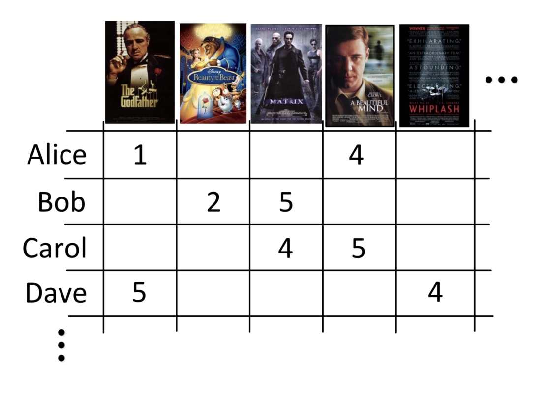
Netflix database consists of about $m \approx 10^6$ users and about $n \approx 25,000$ movies. Users rate movies; the ratings are recorded into matrix $A \in R^{m\times n}$. Only $1\%$ (over 100 million) of the ratings are observed.
\begin{center} \includegraphics[width=0.8\textwidth]{netflix.jpg} \end{center}
Netflix challenge: impute the unobserved ratings for personalized recommendation. (http://en.wikipedia.org/wiki/Netflix_Prize)
$\Omega = \{(i,j) : \text{observed entries}\}$ index the set of observed entries and $P_{\Omega}(\mathbf{M})$ denote the projection of matrix $\mathbf{M}$ to $\Omega$. The problem $$ \min_{\text{rank}(\mathbf{X}) \leq r} \frac{1}{2} \left\| P_{\Omega}(\mathbf{Y}) - P_{\Omega}(\mathbf{X}) \right\|_{F}^{2} = \frac{1}{2} \sum_{(i,j) \in \Omega} (y_{ij} - x_{ij})^{2} $$ is non-convex and hard.
Convex relaxation of the rank minimization problem is: $$ \min_{\mathbf{X}} f(\mathbf{X}) = \frac{1}{2} \|\mathbf{P}_{\Omega}(\mathbf{Y}) - \mathbf{P}_{\Omega}(\mathbf{X})\|_F^2 + \lambda \|\mathbf{X}\|_*, $$ where $\|\mathbf{X}\|_* = \|\sigma(\mathbf{X})\|_1 = \sum_i \sigma_i(\mathbf{X})$ is the nuclear norm.
Majorization step:
$$ \begin{aligned} f(\mathbf{X}) =& \frac{1}{2} \sum_{(i,j) \in \Omega} (y_{ij}-x_{ij})^2 + \frac{1}{2} \sum_{(i,j) \notin \Omega} 0 + \lambda \|\mathbf{X}\|_* \\ \le& \frac{1}{2} \sum_{(i,j) \in \Omega} (y_{ij}-x_{ij})^2 + \frac{1}{2} \sum_{(i,j) \notin \Omega} (x^{(t)}_{ij}-x_{ij})^2 + \lambda \|\mathbf{X}\|_* \\ =& \frac{1}{2} \|\mathbf{X}-\mathbf{Z}^{(t)}\|_F^2 + \lambda \|\mathbf{X}\|_* \\ =& g(\mathbf{X}|\mathbf{X}^{(t)}), \end{aligned} $$ where $\mathbf{Z}^{(t)} = \mathbf{P}_\Omega(\mathbf{Y}) + \mathbf{P}_{\Omega^\perp}(\mathbf{X}^{(t)})$. (Fill in missing entries by the current imputation)
- Minimization step: Rewrite the surrogate function $$ g(\mathbf{X}|\mathbf{X}^{(t)}) = \frac{1}{2} \|\mathbf{X}\|_F^2 - \text{tr}(\mathbf{X}^T\mathbf{Z}^{(t)}) + \frac{1}{2}\|\mathbf{Z}^{(t)}\|_F^2 + \lambda \|\mathbf{X}\|_* $$
Let $\sigma_i$ be the (ordered) sigular values of $\mathbf{X}$ and $\omega_i$ be the (ordered) sigular values of $\mathbf{Z}^{(t)}$. Observe $$ \|\mathbf{X}\|_F^2 = \sum_i \sigma_i^2 \\ \|\mathbf{Z}^{(t)}\|_F^2 = \sum_i \omega_i^2 $$ and by von Neumann's inequality,
$$ \text{tr}(\mathbf{X}^T \mathbf{Z}^{(t)}) \leq \sum_i \sigma_i \omega_i $$
with equality achieved if and only if the left and right singular vectors of the two matrices coincide. Therefore we should choose $\mathbf{X}$ with the same singular vectors as $\mathbf{Z}^{(t)}$ and $$ \begin{aligned} g(\mathbf{X}|\mathbf{X}^{(t)}) =& \frac{1}{2}\sum_i \sigma_i^2 - \sum_i \sigma_i \omega_i + \frac{1}{2}\sum_i \omega_i^2 + \lambda \sum_i \sigma_i \\ =& \frac{1}{2}\sum_i (\sigma_i - \omega_i)^2 + \lambda \sum_i \sigma_i, \end{aligned} $$ with minimizer as $$ \sigma_i^{(t+1)} = \max(0, \omega_i - \lambda) = (\omega_i - \lambda)_+. $$
Algorithm for matrix completion:
Initialize $\mathbf{X}^{(0)} \in\mathbb{R}^{m \times n}$
Repeat
$\mathbf{Z}^{(t)} \leftarrow \mathcal{P}_{\Omega}(\mathbf{Y}) + \mathcal{P}_{\Omega^{\perp}}(\mathbf{X}^{(t)})$
Compute SVD: $\mathbf{U} \mathrm{diag}(\mathbf{w}) \mathbf{V}^{\top} \leftarrow \mathbf{Z}(t)$
$\mathbf{X}^{(t+1)} \leftarrow \mathbf{U} \mathrm{diag}[(\mathbf{w}-\lambda)_+] \mathbf{V}^{\top}$
objective value converges