STAT 207: Advanced Optimization Topics
In general,
unconstrained optimization problems are easier to solve than constrained optimization problems,
equality constrained problems are easier to solve than inequality constrained problems
Inequality constraint - interior point method
We consider the constrained optimization $$ \text{min} f_0(x) $$ subject to $$ \begin{aligned} f_j(x) &\le 0,\quad 1 \leq j \leq m; \\ Ax &= b, \end{aligned} $$ where $f_0,...,f_m: R^n \rightarrow R$ are convex and twice continuously differentiable, and $A$ as full row rank.
Assume the problem is solvable with optimal point $\mathbf{x}^*$ and optimal value $f_0(\mathbf{x}^*) = p^*$.
KKT conditions:
$$ \begin{aligned} \mathbf{A}\mathbf{x}^* = \mathbf{b},\; f_i(\mathbf{x}^*) &\le 0, i=1,..,m \quad \text{(primal feasibility)} \\ \lambda_i^* &\ge 0, i=1,..,m \\ \nabla f_0(\mathbf{x}^*) + \sum_{i=1}^m \lambda_i^* \nabla f_i(\mathbf{x}^*) + \mathbf{A}^T\boldsymbol{\nu}^* &= 0 \quad \text{(dual feasibility)} \\ \lambda_i^*f_i(\mathbf{x}^*) &= 0, \quad i=1,\ldots,m. \end{aligned} $$
Barrier method¶¶
Convert the problem to implicitly include the inequality constraints in the objective and minimize $$ f_0(\mathbf{x}) + \sum_{i=1}^m I_-(f_i(\mathbf{x})) $$ subject to $\mathbf{A}\mathbf{x} = \mathbf{b}$, where $$ I_-(u) = \begin{cases} 0 & \text{if } u \leq 0 \\ \infty & \text{if } u > 0 \end{cases}. $$
And to approximate $I_-$ by a differentiable function $$ \widehat{I}_-(u) = -(1/t)\log(-u), \quad u<0, $$ where $t>0$ is a parameter tuning the approximation accuracy. As $t$ increases, the approximation becomes more accurate.
import numpy as np
import matplotlib.pyplot as plt
import warnings

# Ignore the specific warning
warnings.filterwarnings("ignore", category=RuntimeWarning)

def I_hat_minus(u, t):
    return -(1/t) * np.log(-u)

u = np.linspace(-3, 0, 100)
t_values = [0.5, 1, 2]

for t in t_values:
    plt.plot(u, I_hat_minus(u, t), label=f't={t}')

plt.xlabel('u')
plt.ylabel('I_hat_minus(u)')
plt.legend()
plt.title('Plot of I_hat_minus(u)')
plt.grid(False)
plt.show()

The barrier method solves a sequence of equality-constraint problems $$ \begin{aligned} \min \quad t f_0(\mathbf{x}) - \sum_{i=1}^{m} \log(-f_i(\mathbf{x})) \\ \text{subject to} \quad \mathbf{A}\mathbf{x} = \mathbf{b}, \end{aligned} $$ with increased parameter $t$ at each step and starting each Newton minimization at the solution for the previous value of $t$.
The function $\phi(\mathbf{x}) = - \sum_{i=1}^{m} \log(-f_i(\mathbf{x}))$ is called the logarithmic barrier or log barrier function.
Denote the solution at $t$ by $\mathbf{x}^*(t)$. Using the duality theory, we can show $$ f_0(\mathbf{x}^*(t)) - p^* \le m/t. $$
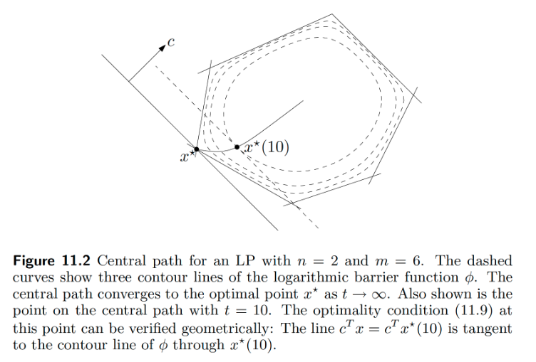
\begin{center} \includegraphics[width=0.8\textwidth]{barrier.jpg} \end{center}
- Barrier method has to start from a strictly feasible point. We can find such a point by solving $$ \text{min} s $$ subject to $$ \begin{aligned} f_j(x) &\le s,\quad 1 \leq j \leq m; \\ Ax &= b, \end{aligned} $$ by the barrier method.
Penalty Method
Unlike the barrier method that works from the interior of the feasible region, the penalty method works from the outside of the feasible region inward.
Construct a continuous nonnegative penalty $p(x)$ that is 0 on the feasible region and positive outside it.
Optimize $$ f_0(x) + \lambda_k p(x) $$ for an increasing sequence $\lambda_k$.
Example (Linear Regression with Linear Constraints) Consider the regression problem of minimizing $\|Y - X\beta \|_2^2$ subject to the linear constraints $V\beta = d$. If we take the penalty function $p(\beta) = \|V\beta - d\|_2^2$, then we must minimize at each stage the function $$ h_k(\beta) = \|Y - X\beta\|_2^2 + \lambda_k \|V\beta - d\|_2^2. $$ Setting the gradient $$ \nabla h_k(\beta) = -2X^T(Y - X\beta) + 2\lambda_k V^T(V\beta - d) = 0 $$ yields the sequence of solutions $$ \beta_k = (X^TX + \lambda_kV^TV)^{-1}(X^TY + \lambda_kV^T d). $$
- Ascent and descent properties of the penalty and barrier methods.
Proposition 16.2.1: Consider two real-valued functions $f(x)$ and $g(x)$ on a common domain and two positive constants $\alpha < \omega$. Suppose the linear combination $f(x) + \alpha g(x)$ attains its minimum value at $y$, and the linear combination $f(x) + \omega g(x)$ attains its minimum value at $z$. Then, $f(y) \leq f(z)$ and $g(y) \ge g(z)$.
- Global convergence for the penalty method.
Proposition 16.2.2 Suppose that both the objective function $f(x)$ and the penalty function $p(x)$ are continuous on $\mathbb{R}^m$, and the penalized functions $h_k(x) = f(x) + \lambda_k p(x)$ are coercive on $\mathbb{R}^m$. Then, one can extract a corresponding sequence of minimum points $x_k$ such that $f(x_k) \le f(x_{k+1})$. Furthermore, any cluster point of this sequence resides in the feasible region $C = \{x : p(x) = 0\}$ and attains the minimum value of $f(x)$ within $C$. Finally, if $f(x)$ is coercive and possesses a unique minimum point in $C$, then the sequence $x_k$ converges to that point.
- Global convergence for the barrier method.
Proposition 16.2.3 Suppose the real-valued function $f(x)$ is continuous on the bounded open set $U$ and its closure $V$. Additionally, suppose the barrier function $b(x)$ is continuous and coercive on $U$. If the tuning constants $\mu_k$ decrease to 0, then the linear combinations $h_k(x) = f(x) + \mu_k b(x)$ attain their minima at a sequence of points $x_k$ in $U$ satisfying the descent property $f(x_{k+1}) \leq f(x_k)$. Furthermore, any cluster point of the sequence furnishes the minimum value of $f(x)$ on $V$. If the minimum point of $f(x)$ in $V$ is unique, then the sequence $x_k$ converges to this point.
Possible defects of of the penalty and barrier methods:
iterations within iterations
choosing the tuning parameter sequence
numerical instability
## jupyter nbconvert --TagRemovePreprocessor.remove_input_tags='{"hide_code"}' --to pdf Opt_top.ipynb